
This project is developed at the University of Wyoming and it is sponsored by the School of Energy resource and the Department of Energy of United States of America. The main objective is the development of numerical methods and models to simulate the injection of CO2 in saline aquifers.
This software is developed in C++ and based on a modular framework in which we can simulate a wide array of mathematical models ranging from the simple biphasic incompressible flow with no mass transfer between phases to the compositional model with very realistic flash computations. Also, for every model we can choose many different numerical methods enabling us to compare the performance of different discretization strategies.
Basically the mathematical equations are divided in three sets of system of equation following a IMPES (Implicit for Pressure, Explicit for Saturation) approach.
For each subsystem we can choose many different models and numerical methods to solve them. Of course, not all models are compatible. For example you cannot run an incompressible biphasic flow with a flash that models a compressible flow. These is the main reason why we say that the interface of this software is not ready for the end user without the support of the developers. This is a software based in serious scientific research and its prerequisites are changing all the time. For example, we plan to incorporate double porosity models, geomechanics and modules that run on GPUs for the next semester.
Corresponding to each subsystem of equations we have three main classes hierarchies acoording to the following UML diagram:
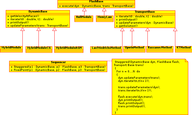
The description of the base classes follows:
The three classes above define the basic interface among the modules. They have many specializations classes corresponding to different numerical methods. For example, for the transport equations, the user can choose the Lax-Friedrichs or Upwind or Russanov or Kurganov-Tadmor and many others classes. All of them are specializations of the TransportBase class. The user supply to the program a configuration file describing which specialization to load for each of the classes (DynamicBase, FlashBase, and Transport Base). When the simulator executes, the modules are created and iterated in time following a sequence alghorithm that advances each module in time exchanging their solutions among themselves. Many different sequence alghorithms with different accurracy and computational costs can be selected by the user, like Fixed-Point type iterations or the simple staggered aproach strategy
The simplified class diagram bellow illustrates the main framework structure of the code
################ Mesh settings. ##############################
# The next parameters build a regular rectangular mesh of
# ElemsX x ElemsY x ElemsZ of dimension DimX x DimY x DimZ

# Number of Elems
NUM_ELEMS_X = 2
NUM_ELEMS_Y = 2
NUM_ELEMS_Z = 2

# Dimension
DIM_X = 1
DIM_Y = 1
DIM_Z = 1


#This key selects the function used to cut the mesh.
#All the cells in the domain of the cut function are flagged
#as visible while the cells outside its domain are set as
#invisible and are never accessed. This makes the mesh be
#usefull in many other geometries other than simple cubes and rectangles
#Options:
# 0) No cut function
# 1) Defines a cylinder inside the mesh  along the Z direction.
#    with circular section inscribed in the plane XY
MESH_CUT_FUNCTION=0

################# DEBUGGING PARAMETERS ####################
#The following flags make the program print some information about the
#mesh.
DEBUG_PRINT_TRIANGULATION = 0


# In the mesh we can  add wells specified as rectangles inside the domain
# All the cells whose barycenters are inside the rectangle are considered
# inside the well. The rectangle is specified with two points P and Q
# such that P(i) < Q(i) i = X,Y,Z. You can specify more than one well.
# If the well is too small to contain at least one barycenter of the
# mesh, the program chooses the nearest barycenter.
WELL_1_PX = 0.5
WELL_1_PY = 0.5
WELL_1_PZ = 0.45
WELL_1_QX = 0.5
WELL_1_QY = 0.5
WELL_1_QZ = 0.4
WELL_1_INJECTION_RATE =


#Fixed Transport Boundary Conditions
#This give the cells where we fix the values of the transport
#primary variables in some cells in order to simulate wells with
#with source terms. For while you can just specifiy two cells
#and only for one variable of the transport equation. The cell
#is specified by a point x,y,z given by the keys S1_FIXED_J_[X,Y,Z]
#and the value to be fixed on that cell is defined in S1_FIXED_J_VALUE
#with J == 1,2,3,4,5,6 indicating the cells
S1_FIXED_1_X=0.5
S1_FIXED_1_Y=0.5
S1_FIXED_1_Z=0.5
S1_FIXED_1_VALUE=1
S1_FIXED_2_X=0.5
S1_FIXED_2_Y=0.5
S1_FIXED_2_Z=0.5
S1_FIXED_2_VALUE=1


############### Transport Equation  Options #############################################
# Chosse the transport module
#	1) LAX FRIEDRICHS for scalar equation
#       2) UPWIND for scalar equation
#       3) Russanov for scalar equation
#       4) Godunov Method
#       5) KT Method
#       6) KT Dimension by Dimension with CUDA
#          If the program is compiled without CUDA an error
#          message will appear
TRANSPORT_MODULE = 1

# Max CFL for the transport methods
MAX_CFL = 0.5

#Choose if the transport module will compute a diffusive step
#This is only relevant for transport modules based on numeric
#methods for hyperbolic equations. In this case, the natural
#way to extend such methods to incorporate diffusion term
#is to use operattor splitting.
# 0 No Diffusive Step
# 1 Mixed Hybrid for compositional
# 2 Double Porosity Diffusive Step
# 3
# 4 Double Porosity Diffusive Step for Obi-Blunt Model
DIFFUSIVE_STEP=0


# Set the boundary conditions for the primary variables of the
#transport method Sn, n=1.....N. Some of the boundary conditions
#options specifies values to be applied at the holes (wells)
#of the mesh like the option 2 bellow. It is important to note that
#if the mesh has no wells then the boundary conditions for the wells
#are ignored. So, for instance, in the case 2 if there is no well,
#we dont have boundary conditions for Sn at all.
#Pay attention that the boundary conditions of the Sn
#must match the velocity fields in the sense
#that we have boundary conditions for Sn if, and only if,
#we have inward flux at that boundary.
#Some boundary conditions need arguments  (ARG1,ARG2,....)
#that are suplied by the keys
#Sn_BOUNDARY_CONDITION_ARG_I for I=1,2,3, n=1...N
#The meaning of the variables Sn depend of the flux function chosen
#(See key FLUX_FUNCTION) For example for biphasic flow S1 means the
#saturation of water, for compositional flow S1 may be the amount
#of moles of water, etc.
#   0) Sn = No boundary condition
#   1) Sn = No boundary condition
#   2) Sn = ARG1 at left boundary
#   3) Sn = 1 at right boundary
#   4) Sn = 1 at front boundary
#   5) Sn = 1 at back boundary
#   6) Sn = 1 at bottom boundary
#   7) Sn = 1 at top boundary
#   8) Fivespot problem where Sn = 1 at the left bottom and
#      the top right corners along all Z. This boundary condition
#      can be seen as two cilinders with infinity height (no Z boundaries)
#      located in the oposite corners. The radius of the cilinder is given
#      by the ARG1 parameter
S1_BOUNDARY_CONDITION = 2
S1_BOUNDARY_CONDITION_ARG_1 =1


#Set the initial value for the primary variables of the flux function
#Sn, n = 0.....Some options for the initial Sn value can have arguments
#that are supllied by the additional keys Sn_INITIAL_ARG_[n,2,3...].
#The meaning of the variables Sn depend of the flux function chosen
#(See key FLUX_FUNCTION) For example for biphasic flow S1 means the
#saturation of water, for compositional flow S1 may be the amount
#of moles of water, etc. In other words the meaning of the variables
# depens on the FLUX_FUNCTION option
#       0) Sn = No Boundary Condition
#	1) Sn = 0
#       2) Sn = Arg1 inside a sphere, Arg2 elsewhere
#  	    x = Argn, {x: |x-center| < radius}
#           x = Arg2, otherwise
#           where radius = Arg3
#                 center =
#	3) The initial condition is a chess board in 3d
#    	   This option needs an extra key called
#    	   S1_INTIAL_ARG_1 which contains the
#    	   data of the chess board. This file
#    	   consist of a sequence of numbers that
#    	   are read into a matrix running in the X,Y,Z
#    	   axis in that order.
#      4)  Sn= Arg1
#
#
#
S1_INITIAL_VALUE = 4
S1_INITIAL_ARG_1=0

#The next fields defines some values used for some options of the
#key S1_INITIAL_VALUE. Please, stay in mind that the meaning of this
#fields depend heavily of the option chosen for the key S1_INITIAL_VALUE
#See the documentation of this key to see the meaning of each of the fields.
#Note that depending of the value chosen for the S1_INITIAL_KEY, the values of
#this fields can be simply ignored by the simulator.
S1_INITIAL_ARG_1 = 0
S1_INITIAL_ARG_2 = 0
S1_INITIAL_ARG_3 = 0
S1_INITIAL_ARG_4 = 0
S1_INITIAL_ARG_5 = 0

#The next key set the porosity field.
#Some options need some arguments that
#are given by the keys POROSITY_ARG_[1...]
#The meaning of the values of each of the POROSITY_ARG
#keys depends of porosity case you choose. In the documentation
#when we refer to Arg1, Arg2.... we mean the keys
#POROSITY_ARG_1, POROSITY_ARG2 and so on.
#The following options are given :
#    1) Porosity field constant: por(x) = Arg1
#    2) Porosity is a chess board specified in a
#       data file. The name of the data file is defined
#       in the key POROSITY_ARG_1. The format of the file
#       is a string specifying the dimensions NUM x NUM x NUM
#	followed by the entries of the porosity field running
#       in X, Y and Z direction respectively.
#       order with the
POROSITY=1

#The arguments for porosity option follows
POROSITY_ARG_1 = "./Por/Por2x2x1.dat"


# The next key defines the flux function used in the transport
# The type of flux defines the number of transport equations of the
# problem
#    1) Scalar Linear flux F(u)=u
#    2) Scalar BUCKLEY-LEVERETT  flux with gravity term
#    3) Scalar Burguers Function
# For more than one hyperbolic equation we have the following options:
#    4) Burguers for the first equation, Linear equation for the second one:
#     	F(S1,S2) = < S1*S1/2, S2 >
#    5) This class implements the flux for the case of CO2 injection in water assuming
#       ideal mixing, incompressibility of the phases, and no evaporation of water into
#       the supercritic CO2 phase, just dissolution of CO2 in water.
#	This is the flux in the article of Obi and Martin Blunt,
#       published in  WATER RESOURCES RESEARCH vol 42. It is defined as
# 	F1(S1=Sc,S2=Cd) =   m_fMob(Sc)*Vdt + K   (1-C)(pw-pc) m_fMobGrav(Sc) g Grad(Z)
#	F2(S1=Sc,S2=Cd) = C*m_fMob(Sc)*Vdt - K C*(1-C)(pw-pc) m_fMobGrav(Sc) g Grad(Z)
#	Where
#		  C = Cd/(1-Sc);
#    		  K = Permeability;
#    		  pw = water specific mass;
#    		  pc = co2 specific mass;
#    		  Cd = Is the fraction volume of the porous media occupied by the dissolved CO2
#    		  Sc = Is the saturation of supercritic CO2
#		  fMob   = Is the bucley leverett mobility
#                 fMobGrav = Is the resulted mobility for the gravity term of the flux
#    6) Flux designed for Simple Black Oil Model of Oil and Gas where
#	Gas can dissolve into oil and oil does not evaporate.
#	The flux is a function of the total moles of each component
#	 OIL (mo), GAS (mg) using Bucley-Leverett Mobility.
#	The flux is given by the expression:
#	Fo(no,ng) =   [m_o^o/volOil * fMobO(So) ]*Vdt
#	Fg(no,ng) =   [m_g^o/volOil * fMobO(So)  +  m_g^g/VolGas * (1-fMobO(So))]*Vdt
#	Where
#	fMob = Bucley Leverret Mobility with
#	GAS Viscosity = Defined By Flash.
#	OIL Viscosity = Defined By Flash
#	So            = Saturation of oil phase.
#    7) Flux designed for CO2 injection in Brine for compositional model.\n\
#       The flux is a function of the total moles of each component
#       (i.e Water,CO2, SALT) using Bucley-Leverett Mobility.
#       The flux is given by the expression:
#       F1(mw,mc,ms) =   [mw_aq/volAqueous * fMob(Sw)  +  mw_gas/VolGas * (1-fMob(Sw))]*Vdt
#       F2(mw,mc,ms) =   [mc_aq/volAqueous * fMob(Sw)  +  mc_gas/VolGas * (1-fMob(Sw))]*Vdt
#       F3(mw,mc,ms) =   [ms_aq/volAqueous * fMob(Sw)]*Vdt
#       Where\n\
#       fMob = Bucley Leverret Mobility with\n\
#        Water Viscosity = %g.\n\
#        CO2 Viscosity   = %g.\n\
#        Sw              = Saturation of water phase.\n\
#        volAqueous      = Volume of aqueous phase at the cell (mw_aq*Vaq + mc_aq*Vcaq + ms_aq Vsaq)\n\
#        volGas          = Volume of supercritic CO2 at the cell\n\
FLUX_FUNCTION = 2


#The next key defines the mobilities functions
#Case 1) Linear Mobility
#Case 2) The normal squared relative permeabilies used
#         by Douglas et al
#Case 4) Mobilities based on the relative permeabilities
#        obtained with Piri-Morteza experiments
RELATIVE_MOBILITY_FUNCTION=1


#For flux functions involving transport in porous media,
#the mobilities generally have as parameters the residual
#saturation of each phase. The fields above set these values
#At the moment these fields are only relevant for fluxes that
#use the general squared mobilities curves adopted by most
#of majority papers in reservoir simulations.
PHASE1_RESIDUAL_SATURATION=0.1
PHASE2_RESIDUAL_SATURATION=0.2


# The next two fields give the viscosities for the phases.
# Important to note that these viscosities' values are only used
# for the flux functions that use Bucley-Leverett fluxes.
# S1_VISCOSITY is the viscosity of the phase belonging to the
# solution S1 and S2_VISCOSITY is the same thing for the phase
# belonging to the variable S2
S1_VISCOSITY = 1
S2_VISCOSITY = 20


# The next Two  fields give the specific weight of the fluids belonging
# to the concentrations S1 and S2
# This values are used to generate the flux terms related with
# the gravity. Currently the gravity term is only used for the
# bucley-leverett flux  function (FLUX_FUNCTION = 2),
# in the other options the gravity term is neglected in both
# modules (transport and dynamic).
S1_DENSITY = 1
S2_DENSITY = 1

#Gravity acceleration
GRAVITY=10

#Cappillary Pressure Function
# 0) Zero Cappillar Pressure
#    fPc(S1) = 0
# 1) Linear Cappillar Pressure where
#    fPc(0) = ARG1
#    fPc(1) = ARG2
# 2) The capillar pressure given by
#    Pc(s) = eta ((s-Sr1)^-2 - tau (1-s)^-2)\
#    where
#    eta=ARG1
#    tau=Sr2^2 * (1-Sr2-Sr1)^2\
#    Sr1=PHASE_1_RESIDUAL_SATURATION
#    Sr2=PHASE_2_RESIDUAL_SATURATION
#    Capillary Pressure Threeshold=ARG2
#
#    Note that this functions goes to infinity as s goes to Sr1
#    The capillary Threshold gives the maximum admissible
#    capillary pressure, beyond this value the function just
#    return the threshold specified in ARG2. If such argument
#    is not specified in the config file  than the  default value
#    is INFINITY which means that there is no capillary Threshold at all
CAPILLARY_PRESSURE=0
CAPILLARY_PRESSURE_ARG_1=0
CAPILLARY_PRESSURE_ARG_2=200e+5

#Capillary Pressure Function for Matrix Blocks
# 0) Zero Capillar Pressure
#    fPc(S1) = 0
# 1) Linear Capillar Pressure where
#    fPc(0) = ARG1
#    fPc(1) = ARG2
# 2) Capillary Pressure J. Douglas et al.
#    ARG1 is eta
#    ARG2 Is the saturation threshold used to calculate the
#    pc inverse. If the saturation is less than this value the pc
#    inverse is calculated with the bisection alghorithm wich is
#    a very expensive procedure. If the saturation is beyond this
#    value, then we use linear interpolation.
#         Note, s_min=srw, s_max=1-sro and Pc_max=Pc(s_Pc_max)
#    ARG3 is the numbers of equally spaced used subintervals to be used for
#         linear interpolation of P on [0,Pc_max]
#         Default value is 100 if ARG3 in not given
#    ARG4 is the largest Capillary pressure allowed by Flash Calculation
#         when relevant. Default value if not set is INFINITY
MB_CAPILLARY_PRESSURE = 2
MB_CAPILLARY_PRESSURE_ARG_1 = 300  #300 #N/m^2 (etha)
MB_CAPILLARY_PRESSURE_ARG_2 = 0.25
MB_CAPILLARY_PRESSURE_ARG_3 = 1000
#MB_CAPILLARY_PRESSURE_ARG_4 = 5000

#Capillary Pressure Function Case (2) makes use of a Bisection Method for
#calculation of inverse function values. The following key controls the
#numerical tolerance for this procedure. Default value if not set is 10^(-6).
BS_METHOD_TOLERANCE = 1.0e-6


####################  FLASH MODULE OPTIONS ##################################
# Wich flash module we want to load
# 1) Dummy flash, it makes no computations
# 2) Henry Law flash
# 3) The Henry Law flash but for the Obit Blunt model
#    defined in terms of saturation of CO2 and Concentration of
#    CO2 in water  instead of moles per pore volume usually
#    used in compositional models
# 4) The real Flash code made by Allan and Piri.
#    It assumes a constant temperature given by the key
#    TEMPERATURE. S1=WATER MOLES, S2=CO2 MOLES, S3=SALT MOLES
# 5) Simple Black Oil Model for OIL and GAS where only gas\n	\
#    can dissolve in oil. The units of the simulator for this
#    flash is:
#
#    distance ft
#    time     days
#    Pressure PSI
#
#    This flash override the viscosities values given to
#    the mobility functions such that they depend on
#    the pressure.
#    "John B Bell, Gregory R. Shubin, John Trangestein
#    METHOD FOR REDUCING NUMERICAL DISPERSION IN TWO
#    PHASE BLACK OIL RESERVOIR SIMULATION, Journal of
#    Computational Physics 65, 71-106 1986"
FLASH_MODULE = 5


#This options are specific to the flash module that computes the henry law
#HENRY_COEFFICIENT =
#APPARENT_CO2_MOLAR_VOLUME =
#R=
#TEMPERATURE=
#GAS_MOLAR_VOLUME=
#LIQUID_MOLAR_VOLUME=


####################  Dynamic Module Options ##################################
# These option control which dynamics modules are loaded.
#    1) Use a module which always gives a stationary constant velocity field (no changes in
#       the velocity field along the time). This is used specially for testing the transport module and
#       there are many possible velocity fields we can choose each one associated with a specific value
#       for the CONST_VELOCITY_FUNCTION key
#    2) Read velocities from a file described by the key VELOCITY_FILE.
#       This file describes a velocity field in 2D and it is projected in a 3D mesh
#       with just one element at Z direction. So to use this option be sure that the
#       key NUM_ELEMS_Z is always 1. The format of the file is one line per cell.
#       The cells are reading in a grid form, from x---xend, y---yend and for each cell
#       (or for each line in the file) we have the normal velocities of the left
#       right down and up velocities.
#
#    3) This module solves the pressure equation resulted from compositional model. The
#        pressure equation is
#
#	B dp/dt + div(u) = f
#       u = -KmobT(Sw)Grad(P)
#
#       Please see Mathematical Structure of Compositional Reservoir Simulation,
#       Trangenstein, John Bell SIAM Vol 5 819-845,  September of 2009.
#	This option uses the keys PRESSURE_INITIAL_VALUE for the initial condition
#       of the pressure, DYNAMIC_DEBUG_LEVEL and PRESSURE_BOUNDARY_CONDITIONS
#       Pressure must be given in N/m2
#     4)  The system is solved by a iterative solver using the schur complement technique.
#       The mixed formulation with RT results in the following system:
#        | M  B| |V| = G
#        | BT 0| |P|   F
#	Where V and P are the degrees of freedom of the velocity and pressure respectively.
#       The secret is to solve first for pressure than for velocitie. Solvin the system
#       for pressure we have BT*Inv(M)*B*P = BT * Inv(M) * G - F. To solve we use
#       the CG method with the matrix BT*Inv(M)*B. Each multiplication of the matrix
#       is done with another inner CG method to calculate Inv(M).
#    5) Compositional model considering all the terms of the pressure equation.
#    6) This module use the hybrid formulation to find solution of incompressible biphasic flow
#    7) Method that uses cappillary pressure defining the system in terms of
#       pw.
#    9) Hybrid Formulation with Domain Decomposition Method with UMFPAC
#       (Enabled Only with MPI)*
#   10) Hybrid Formulation with Domain Decomposition Method with CG and AGM
#       (Enabled Only with MPI)*
#   11) Solve the elliptic equation for the pressure using post processing
#       to increase the conservative properties of the resulting velocity fields (Murad and Loula)
#Obs: Please note that, unless indicated, all the dynamic modules run in
#sequential code. So if you compile the code with the MPI support and want
#to use a sequential dynamic module, be sure to run it using just one process.
DYNAMIC_MODULE = 6

# This key set the cappillary pressure with the matrix block.
# It is relevant only for case DYNAMIC_MODULE=8
POTENTIAL_C=2.5


# This key controls which velocity field is loaded for the case that
# DYNAMIC_MODULE = 1. If the DYNAMIC_MODULE key is different of
# 1 this key value has no effect.
#   1)Undimensional Transport test in X direction: Velocity = <1,0,0>
#   2)Undimensional Transport test in X direction: Velocity = <-1,0,0>
#   3)Undimensional Transport test in Y direction: Velocity = <0,1,0>
#   4)Undimensional Transport test in Y direction: Velocity = <0,-1,0>
#   5)Undimensional Transport test in Z direction: Velocity = <0,0,1>
#   6)Undimensional Transport test in Z direction: Velocity = <0,0,-ARG1>
#   7)Unidimensional Transport test with two tracks
#   		     Velocity = <1,0,0> in the upper half Y > DIM_Y/2.0
#		     Velocity = <0.2,0,0> in the lower half Y < DIM_Y/2.0
#   8)Velocity = 0
CONST_VELOCITY_FUNCTION=8


#This option is used only if DYMAMIC_MODULE==2
#This key specifies which file the dynamic module should read
#to generate the velocity fields
VELOCITY_FILE="./"


#Type of Linear solver
#     1) Direct Linear Solver UMFPACK for Sparse
#        Matrices with LU decomposition
#     2) CG solver with AGM preconditioning for
#        Sparse Matrices
#

LINEAR_SOLVER=1


#The key bellow when relevant the number of
#iterations and tolerance of  the linear solver used
#by the dynamic modules. Some parameters are only considered
#when we select iterative linear solvers  methods.
SOLVER_NUM_ITERATIONS = 10000
SOLVER_TOLERANCE = 1.E-05

#The next options are relevant only for the modules that use
#Domain Decomposition in special the method provided in the Oscar Osmay Thesis
#1)The  tolerance used to check for local convergence if the data beetween
#two iterations change less than this parameter among all subdomains than
#the iteration is over
#2) The B parameter is  used in the robin conditions between subdomains.
#(See Oscar's Thesis). The robin condition is  Tr + B*ur = Tl + B*ul,
#where ur and ul are the velocity between two adjacent
#subdomains and Tr, Tl are the trace of the pression
DDM_TOLERANCE=1.E-05
DDM_B_PARAMETER=0.25


#The above key is to set the amount of debugging information printed by the dynamic modules.
#The following is a list of what informations are printed for each dynamic module
# DYNAMIC_MODULE = 1 (No debug information)
# DYNAMIC_MODULE = 2
#   DEBUG_LEVEL = 1 : Print pression
# DYNAMIC_MODULE = 3
#   DEBUG_LEVEL = 1 : Convergence information about the outter cg method
#   DEBUG_LEVEL = 2 : Convergence information about the outter cg method and the
#                     inner one wich is used to solve Inv(M). See documentation for the
#                     DYNAMIC_MODULE=3 option
DYNAMIC_DEBUG_LEVEL = 2


# Boundary conditions for the pressure and the velocity.
# The following options are available. Please, note that
# the Velocity function vel(x) bellow describes the size of the normal
# component of the velocity along the boundary. Some of the
#boundary conditions options available dont  include boundary conditions
# at the wells. In the case that we have wells and we choose such boundary
# conditions, the boundaries of the well will not be setted witch implies
# boundary condition for pressure equal to zero in the well, since
# we are using hybrid formulation.
# 1) p = 0 at the boundaries of the reservoir;
# 2) vel(x) =  at left boundary
#    p = ARG2 at right boundary
#    vel(x) = 0 at the other domain boundaries
# 3) p = ARG1 at the  left boundary (X=0)
#    p = ARG2 at the right boundary.
#    Null flux at other boundaries;
# 4) vel(x) = 0 in all boundary
#    For this kind of condition is sometimes usefull to specify a reference pressure
#    in the domain, otherwise the problem is not well posed. I.e We have many solutions
#    for the pressure that are different by a constant. To solve that
#    the user can specify a value for pressure to be stored in the bottrom front left corner
#    The value of this reference pressure is specified in PRESSURE_BOUNDARY_CONDITION_ARG_1 in case this argument
#    is not present. No reference pressure is taken into account
# 5) Unidimensional pression condition in X direction
#    vel(x) = 0 at the top, bottom, front and back sides
#    p=Arg1, p = Arg2 in the right and left bottom
# 6) Unidimensional pression condition in Y direction
#    vel(x) = 0 at the top, left, right and back sides
#    p=Arg1, p = Arg2 in the front and back sides
# 7) Unidimensional pression condition in Z direction
#    vel(x) = 0 at the left, right, front and back sides
#    p=Arg1, p = Arg2 in the bottom and up faces
# 8) Fivespot problem with injection well at the front left
#    corner and production well at the back right corner.
#    The wells' radius is specified in the ARG_3, The velocity
#    at the injection well is defined by ARG_1 and the pressure
#    in the production well is set in ARG_2
# 9) vel(x) = <-ARG1,0> at upper boundary
#    p = ARG2 at bottom boundary
#    vel(x) = 0 at the other domain boundaries
# 100) the boundary conditions in the case a mesh is a cylinder (MESH_CUT_FUNCTION=1)
#      Pressure = ARG1 is prescribed in the bottom, Velocity given by <0,0,-ARG2> is
#      prescribed in the upper side, and velocity is null along
#      the revolution surface (the side of the cilinder)


PRESSURE_BOUNDARY_CONDITIONS=100
PRESSURE_BOUNDARY_CONDITIONS_ARG_1=0
PRESSURE_BOUNDARY_CONDITIONS_ARG_2=0

#This option choses the initial condition for the pressure
#This option is only relevant for those dynamic modules that
#implement compressible models where we have time diferentiation
#of the pressure such as the Compositional model. The options
#are:
# 1) Pressure is constant and equal to PRESSURE_INITIAL_VALUE_ARG_1
PRESSURE_INITIAL_VALUE=1
PRESSURE_INITIAL_VALUE_ARG_1=80e+5


# This option choses the permeability field
# 1) Permeability K = PERMEABILITY_ARG_1
# 2) Permeability is a chess board in 3d
#    This option needs an extra key called
#    PERMEABILITY_FILE which contains the
#    data of the chess board. This file
#    consist of a sequence of numbers that
#    are read into a matrix running in the X,Y,Z
#    axis in that order.
# 3) Permeability is a chess board in 3d
#    This option needs an extra key called
#    PERMEABILITY_FILE which contains the
#    data of the chess board. This file
#    has the same format as option 2. The
#    only difference is that it reads the
#    numbers in the file creating a
#    gaussian distribution assigning the
#    value of the permeability as
#    K(dd) = C0exp(c*dd) where dd represents
#    a number read from the file and c, C0 are
#    constants that are set such that the distribution
#    has the coeficient of variance (CV) and media given
#    by the keys PERMEABILITY_MEDIA, PERMEABILITY_CV.
PERMEABILITY=1
PERMEABILITY_ARG_1=1

# The data to read the permeability values.
# This key is only considered when the PERMEABILITY
# key is set to 2.
PERMEABILITY_FILE = "./Permeability/K1.dat"

# The media and the coeficient of variance (CV = Variance/Media) are
# set with the keys bellow. This values has only use when we set
#PERMEABILITY=3
PERMEABILITY_CV = 1
PERMEABILITY_MEDIA = 1


##########################DISPLACEMENT OPTIONS ######################
#The options bellow control the BC for the geomechanic in case the
#dynamic module has some geomechnical coupling. Here we specify condition
#for the displacement U and tension applied in the reservoir
#The BC is controlled by the key DISPLACEMENT_BOUNDARY_CONDITIONS that
#can have the following values
#
# 1) The box send pistol. The reservoid is inside an undeformable box
#     open only on the top where we prescribe a compressiong tension given by
#     ARG1.
#     U0(x) = 0 at LEFT and RIGHT
#     U1(x) = 0 at FRONT and BACK
#     U3(x) = 0 at Bottom
#     Tension = ARG1 at UP
#
# 2) Uniaxial Tensile Test in one of the axis. Arg1 is a string with possible
#    values "X+" "X-" "Y+" "Y-" "Z+" "Z-" indicatin the axis X,Y,Z and if the
#    load is in the negative side or positive side of the reservoir
#    So X+ is a uniaxial tensile test in X direction in the RIGHT BOUNDARY
#       X- is a uniaxial tensile test in X direction in the LEFT BOUNDARY
#    and so on. In the oposite side we prescribe displacement 0 in all
#    dimensions.
#    In all other boundaries, we prescribe 0 Tension (The natural BC).
#    The tension applied is given in ARG2. A positive value denotes extension,
#    a negative value indicates compression

DISPLACEMENT_BOUNDARY_CONDITIONS=1
DISPLACEMENT_BOUNDARY_CONDITIONS_ARG_1="X+"
DISPLACEMENT_BOUNDARY_CONDITIONS_ARG_2=10


#The elastic constants values for YOUN modulus and poisson value
YOUNG_COEFFICIENT=100
POISSON_COEFICIENT=0

############################# SEQUENCER OPTIONS ########################

# Select the alghorithm used to iterate the transport and the dynamic module
# in time
#   0) The sequencer iterates just the dynamic module one time and quit. This option
#      is used to debug the dynamic modules.
#   1) The sequencer iterates the dynamic module only one time just to get a velocity
#      field. Then it iterates the transport until the end of the simulation. This is
#      a option made for the development team to test the transport modules.
#   2) The sequencer iterates the dynamic module first and then the transport module
#      in sequence. The number of iterations of the dynamic moudle is controlled by the
#      key N_DYNAMIC_ITERATIONS
#   3) It is sequence method created for flash calculations. It is very similar to the
#      sequence alghorithm 2. It  iterates the dynamic module first and then the transport module
#      doing flashes calculations for each iteration of the transport module. You can control the
#      sequence alghorithm using the  parameter  N_DYN_ITERATION
#   4) Diffusive Step test.
#   5) Transient Dynamic Module test. A transient dynamic module is the one that has partial
#      derivatives in time in their equations. The Staggered Alghorithm just advances the
#      dynamic module keeping the transport solution stationary at time 0
#
SEQUENCE_ALGORITHM = 3

#Number of iteratios of the dynamic modules during the simulation
N_DYN_ITERATIONS = 20

#This key control the maximum allowed number of transport iterations
#per dynamic iteration. This key is optional and it is relevant only
#for the SEQUENCE_ALGHORITHM 3
TRANSPORT_PER_DYNAMIC_STEPS=100;


#This key control the tolerance of
#maximum allowed number of transport iterations.
#For example if TRANSPORT_PER_DYNAMIC_STEPS  is 3
#and TRANSPORT_PER_DYNAMIC_STEPS_TOLERANCE=1;
#the alghorithm will always try to adust the time step
#of the dynamic step for 3 transport equations but
#will accept  4 transport iterations per
# 1 dynamic iteration.
#This key is optional and it is relevant only
#for the SEQUENCE_ALGHORITHM 3
TRANSPORT_PER_DYNAMIC_STEPS_TOLERANCE=1;


#################### Time Setting #########################
#Final time of the simulation
END_TIME = 0.2


##################### Number of Outputs ######################
# The number of times durign the simulation that the program outputs the solution.
# For example if N_OUTPUTS = 5 and END_TIME=5, the program will plot the solution
# for the instants 1,2,3,4,5, if N_OUTPUTS=10 then the solution is outputted in
# 0.5, 1, 1.5, 2, 2.5 and so on
N_OUTPUTS = 2
HDF5_OUTPUT = "./data.hdf"
| deal.II is an acronym for Differential Equations Analysis Library. This library is a lesson about how to design and use object orientation for finite elements. We basically use their linear and base packages together with some finite elements in the parametric configuration. Since we use structured meshes without local refinement, due to performance factors we could not use the full extent of this powerfull and well documented library. | |
 |
UMFPACK is developped by Tim Davis at University of Florida. It is a library to apply LU decomposition for sparse matrices. It is excellent for small problems and used by us mainly to compare with the solution of iterative solvers. Unfortunately the memory consumption of this solver is too high for the dimension of our real simulations. This mainly happens because the LU decomposition tends to destroy the sparsity pattern of the original linear system despite the incredible efforts of his author to minimize that. In terms of direct solvers, the UMFPACK can be considered a state of art achievement. |
| HDF5 This is a library to store scientific data in an hierarchial way. To correct interpret and debug the simulation results, the software needs to output a wide range of vector and scalar data fields for different time steps. The HDF5 offers a way to store all this data into one unique file in a very organized way similar to the directory trees in a file system. It offers a very well designed API in C and C++. | |
| VTK The visualization toolkit is used to visualize the data. This is done through a program we developed called Mplot. The Mplot receives as input the HDF5 format file produced by our simulator and a script that instructs the Mplot how to plot the data. Is a scheme inspired from the GnuPlot program. In fact the script language we defined is very simular to the former. MPlot can be considered a GnuPlot with VTK as its graphic engine. | |
 |
CUDA is a low level library developed by NVidia to use Graphical Process Units (GPU's) for scientific computing. The use of GPU's showed outstanding performance for our applications specially for the flash computations with speedups factors near 100. In particular we highlight the use of the algebraic multigrid alghorithm to solve the positive definite system of the pressure equations. The implementation of this alghorithm for CUDA was developed by Manfred Liebmann who we have the pleasure to work with us for a short period. His code and all the framework he developed is a separate project at Source Forge called Parallel Toolbox . |